FrequencySystemBuilder

This class handles frequency-domain analysis of linear electric systems.

Features

Supports tension and intensity sources
Models inductive and resistive mutuals
Detects and couples multiple subsystems
Accepts arbitrary complex impedances and mutuals
Constructs sparse linear systems in COO format

Tip

Some solvers do not support complex-valued systems. Use cast_complex_system_in_real_system from utils.py to convert an n-dimensional complex system into a 2n-dimensional real system.

Example

We would like to study the following system:

Multiple system

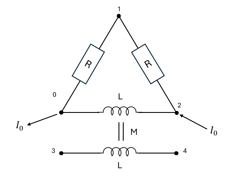
This can be defined in the following manner. We took R=1, L=1 and M=2.

import numpy as np
from scipy.sparse.linalg import spsolve
from ElecSolver import FrequencySystemBuilder


# Complex and sparse impedance matrix
# notice coil impedence between points 0 and 2, and coil impedence between 3 and 4
impedence_coords = np.array([[0, 0, 1, 3], [1, 2, 2, 4]], dtype=int)
impedence_data = np.array([1, 1j, 1, 1j], dtype=complex)

# Mutual inductance or coupling
# The indexes here are the impedence indexes in impedence_data
# The coupling is inductive
mutuals_coords = np.array([[1], [3]], dtype=int)
mutuals_data = np.array([2.0j], dtype=complex)

electric_sys = FrequencySystemBuilder(
    impedence_coords,
    impedence_data,
    mutuals_coords,
    mutuals_data,
)

# Add source (current source here)
electric_sys.add_current_source(intensity=10, input_node=2, output_node=0)

# Set ground
# 2 values because one for each subsystem
electric_sys.set_ground(0, 3)

# Build system
electric_sys.build_system()

# Get and solve the system
sys, b = electric_sys.get_system()
sol = spsolve(sys.tocsr(), b)
frequencial_response = electric_sys.build_intensity_and_voltage_from_vector(sol)

# We see a tension appearing on the lonely coil (between node 3 and 4)
print(frequencial_response.potentials[3] - frequencial_response.potentials[4])

Adding a Parallel Resistance

We want to add components in parallel with existing components, for instance inserting a resistor in parallel with the first inductance between nodes 0 and 2.

Parallel system

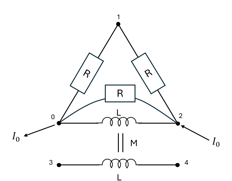
In Python, simply add the resistance to the list of impedances in the first lines of the script:

import numpy as np
from scipy.sparse.linalg import spsolve
from ElecSolver import FrequencySystemBuilder


# We add an additional resistance between 0 and 2
impedence_coords = np.array([[0, 0, 1, 3, 0], [1, 2, 2, 4, 2]], dtype=int)
impedence_data = np.array([1, 1j, 1, 1j, 1], dtype=complex)

# No need to change the couplings since indexes of the coils did not change
mutuals_coords = np.array([[1], [3]], dtype=int)
mutuals_data = np.array([2.0j], dtype=complex)

Gradient Backpropagation

FrequencySystemBuilder can backpropagate gradients from S and rhs to model parameters.

This enables gradient-based optimization loops directly on source values or component data.

Example: Optimize a Voltage Source

In this example, we optimize the voltage source value so the system response matches a target solution.

import numpy as np
from scipy.sparse.linalg import spsolve
from ElecSolver import FrequencySystemBuilder

## sparse python res matrix
impedence_coords = np.array([[0, 0, 1], [1, 2, 2]], dtype=int)
impedence_data = np.array([1, 1, 1], dtype=complex)

## mutuals
mutuals_coords = np.array([[0], [1]], dtype=int)
mutuals_data = np.array([2.0j], dtype=complex)

electric_sys = FrequencySystemBuilder(
    impedence_coords,
    impedence_data,
    mutuals_coords,
    mutuals_data,
)

# Target solution is the solution of the system when voltage=5
electric_sys.add_voltage_source(voltage=10, input_node=1, output_node=0)
electric_sys.set_ground(0)
electric_sys.build_system()

## Getting system
sys, b = electric_sys.get_system(sparse_rhs=True)
sol = spsolve(sys.tocsr(), b.todense())

# Target solution (artificially made by setting voltage_source_data = np.array([5], dtype=complex))
sol_target = np.array([
    -1.66666667 + 1.66666667j,
    -0.83333333 + 1.66666667j,
    0.83333333 - 1.66666667j,
    2.5 - 3.33333333j,
    0.0 + 0.0j,
    5.0 + 0.0j,
    4.16666667 + 1.66666667j,
])

for _ in range(3000):
    ## Computing gradients of squared error with respect to b
    db = 2 * spsolve(sys.tocsr().conj().T, sol - sol_target)
    drhs = db[b.row]

    ## Backpropagate gradients from drhs to voltage_source_data
    gradients = electric_sys.backpropagate_gradients(drhs=drhs)
    ## Performing gradient descent on voltage_source_data
    electric_sys.voltage_source_data = (
        electric_sys.voltage_source_data - 0.01 * gradients.voltage_source_data
    )

    ## After updating voltage_source_data, rebuild the system to update sys and b
    electric_sys.build_system()
    sys, b = electric_sys.get_system(sparse_rhs=True)
    sol = spsolve(sys.tocsr(), b.todense())

## Checking whether we converged to the right solution
np.testing.assert_allclose(electric_sys.voltage_source_data, np.array([5], dtype=complex))

For additional backpropagation examples, see tests/test_gradients.py.

Note

Although providing the backpropagation feature, ElecSolver does not provide an automatic differentiation mechanism. You may use and wrap Elecsolver in automatic differentiation libraries, such as autograd, jax, PyTorch and many more, to avoid the hassle of computing gradients manually.