TemporalSystemBuilder

This class models time-dependent systems using resistors, capacitors, coils, and mutuals.

Features

Supports tension and intensity sources
Models inductive and resistive mutuals
Detects and couples multiple subsystems
Accepts resistances, capacities, and coils
Constructs sparse linear systems in COO format

Example

We would like to study the following system:

Temporal system

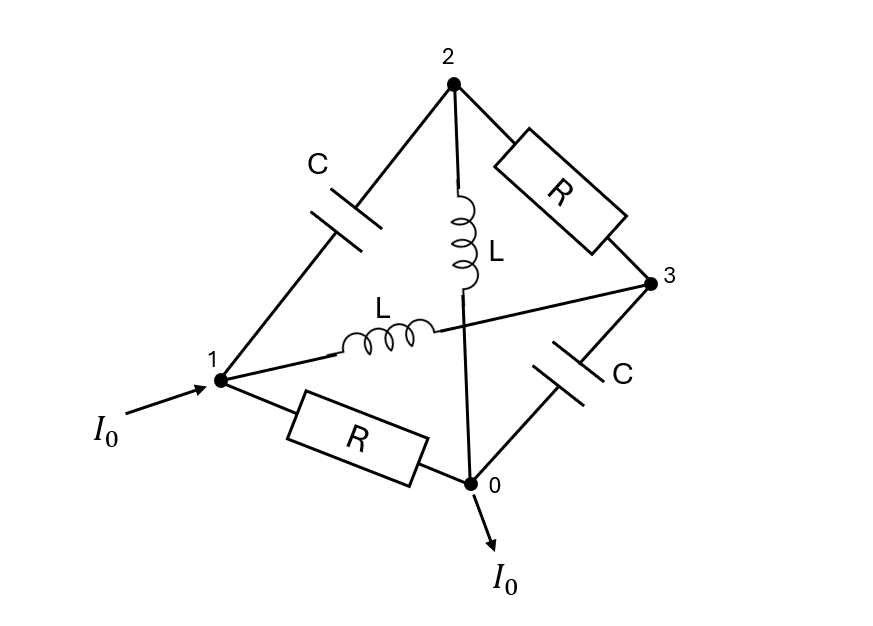
With R=1, L=0.1, C=2 this gives:

import matplotlib.pyplot as plt
import numpy as np
from scipy.sparse.linalg import spsolve
from ElecSolver import TemporalSystemBuilder

## Defining resistances
res_coords = np.array([[0, 2], [1, 3]], dtype=int)
res_data = np.array([1, 1], dtype=float)

## Defining coils
coil_coords = np.array([[1, 0], [3, 2]], dtype=int)
coil_data = np.array([0.1, 0.1], dtype=float)

## Defining capacities
capa_coords = np.array([[1, 3], [2, 0]], dtype=int)
capa_data = np.array([2, 2], dtype=float)

## Defining empty mutuals here
mutuals_coords = np.array([[], []], dtype=int)
mutuals_data = np.array([], dtype=float)

res_mutuals_coords = np.array([[], []], dtype=int)
res_mutuals_data = np.array([], dtype=float)

## Initializing system
elec_sys = TemporalSystemBuilder(
    coil_coords,
    coil_data,
    res_coords,
    res_data,
    capa_coords,
    capa_data,
    mutuals_coords,
    mutuals_data,
    res_mutuals_coords,
    res_mutuals_data,
)

## Add source
elec_sys.add_current_source(10, 1, 0)

## Setting ground at point 0
elec_sys.set_ground(0)

## Build system
elec_sys.build_system()

# Getting initial condition system
S_i, b = elec_sys.get_init_system()
sol = spsolve(S_i.tocsr(), b)

# Get system (S1 is real part, S2 derivative part)
S1, S2, rhs = elec_sys.get_system()

## Solving using implicit Euler scheme
dt = 0.08
vals_res1 = []
vals_res2 = []

for _ in range(50):
    temporal_response = elec_sys.build_intensity_and_voltage_from_vector(sol)
    vals_res1.append(temporal_response.intensities_res[1])
    vals_res2.append(temporal_response.intensities_res[0])
    sol = spsolve(S2 + dt * S1, b * dt + S2 @ sol)

plt.xlabel("Time")
plt.ylabel("Intensity")
plt.plot(vals_res1, label="intensity res 1")
plt.plot(vals_res2, label="intensity res 2")
plt.legend()
plt.savefig("intensities_res.png")

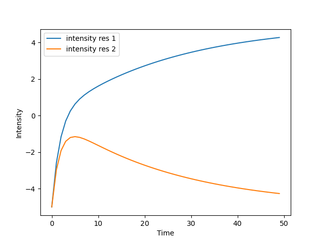
This outputs the following graph that displays the intensity passing through the resistances:

Intensity through resistances

Gradient Backpropagation

TemporalSystemBuilder can backpropagate gradients from S_init, S1, S2, and rhs to component parameters.

This makes it possible to optimize circuit parameters with gradient descent in loops where the solver output is compared to a target.

Example: Optimize Capacitor Values

In this example, we optimize capa_data so the solution at t=0.8 matches a target response.

import numpy as np
from scipy.sparse.linalg import spsolve
from ElecSolver import TemporalSystemBuilder

## Simple tetrahedron
res_coords = np.array([[0, 2], [1, 3]], dtype=int)
res_data = np.array([1, 1], dtype=float)

coil_coords = np.array([[1, 0], [2, 3]], dtype=int)
coil_data = np.array([1, 1], dtype=float)

capa_coords = np.array([[1, 2], [3, 0]], dtype=int)
capa_data = np.array([1, 1], dtype=float)

## mutuals
mutuals_coords = np.array([[], []], dtype=int)
mutuals_data = np.array([], dtype=float)

res_mutuals_coords = np.array([[], []], dtype=int)
res_mutuals_data = np.array([], dtype=float)

elec_sys = TemporalSystemBuilder(
    coil_coords,
    coil_data,
    res_coords,
    res_data,
    capa_coords,
    capa_data,
    mutuals_coords,
    mutuals_data,
    res_mutuals_coords,
    res_mutuals_data,
)
elec_sys.add_current_source(10, 1, 0)
elec_sys.set_ground(0)
elec_sys.build_system()

## Getting initial condition system
S_i, rhs = elec_sys.get_init_system(sparse_rhs=True)
## Getting temporal systems
S1, S2, rhs = elec_sys.get_system(sparse_rhs=True)
## Solving initial condition system
sol_init = spsolve(S_i.tocsr(), rhs.todense())

## Time iteration with euler implicit scheme for 1 timestep
dt = 0.8
B = rhs * dt + S2 @ sol_init
A = S2 + dt * S1
sol = spsolve(A, B)

# Target solution (artificially made by setting capa_data = np.array([0.1, 1], dtype=float))
sol_target = np.array([
    3.24786325,
    -1.1965812,
    -6.16809117,
    0.61253561,
    0.58404558,
    -2.63532764,
    0.0,
    6.16809117,
    2.10826211,
    1.4957265,
])

for _ in range(1000):
    ## computing gradients
    dB = 2 * spsolve(A.T, sol - sol_target)
    ## chain rule for gradients of capa_data (S2 appears twice in the computation graph)
    dS2 = -(dB[S2.row] * sol[S2.col]) ## Gradient from the solver (A\B) to S2
    dS2 += dB[S2.row] * sol_init[S2.col] ## Gradient from the solver (A\B) to S2 through B

    ## Backpropagate gradients from dS2 to capa_data
    gradients = elec_sys.backpropagate_gradients(dS2=dS2)
    ## Change the values of capa_data using gradient descent
    elec_sys.capa_data = elec_sys.capa_data - 0.01 * gradients.capa_data

    ## After updating capa_data, rebuild the system to update S1, S2 and rhs
    elec_sys.build_system()
    S1, S2, rhs = elec_sys.get_system(sparse_rhs=True)
    ## Recompute solution with euler implicit scheme
    B = rhs * dt + S2 @ sol_init
    A = S2 + dt * S1
    sol = spsolve(A, B)

## Checking whether we converged to the right solution
np.testing.assert_allclose(elec_sys.capa_data, np.array([0.1, 1], dtype=float))

For additional backpropagation examples, see tests/test_gradients.py.

Note

Although providing the backpropagation feature, ElecSolver does not provide an automatic differentiation mechanism. You may use and wrap Elecsolver in automatic differentiation libraries, such as autograd, jax, PyTorch and many more, to avoid the hassle of computing gradients manually.